How deep learning mimics the human brain, and can open the door to the creation of truly intelligent machines.
by Izer Onadim
Abbreviations used, in alphabetical order:
AI – Artificial Intelligence
ANN – Artificial Neural Network
DL – Deep Learning
ML – Machine Learning
MLP – Multi-Layer Perceptron
MNIST – Modified National Institute of Standards and Technology
MSE – Mean Squared Error
NN – Neural Network
Since the invention of the Turing Machine in 1936 by mathematician Alan Turing, the field of tasks once considered to be solely the domain of humans, and yet are now delegated to computers has grown at an increasing rate. Subsequently, this led to the idea that machines could also take over from humans in the domain of intellect. It was this idea that created the research field of artificial intelligence, helmed by “Computing Machinery and Intelligence”, a 1950 paper by Turing. In this paper, he theorised that computers would one day become so powerful that they would gain the ability to think. He devised the now famous “Turing Test”1, in which a judge sits at a computer, and types questions to two different individuals, one of which is human, and the other a machine. If this judge cannot tell which of the individuals is human and which is not, then the machine is classed as intelligent. The following essay will demonstrate that in his claim that computers would be able to think if only they became powerful enough, Turing was wildly wrong, and that whilst the Turing test is a useful metric by which we can measure our progress in AI, it is a completely inadequate classifier of intelligence.
A good rebuttal of Turing’s idea that conventional computers could become intelligent, given enough power and complex code, is a thought experiment designed by philosopher John Searle2. It describes a room in which there is an English speaker with a large book of instructions, written in English, that explain how to manipulate and sort Chinese characters, without explaining their meanings. A slip of paper with a story and comprehension questions, all written in Chinese is passed through a slot in the wall of the room, and the man uses the instruction set that he was given to manipulate the characters from the story into precise answers to the questions; he simply follows instructions and has no understanding of what the characters mean. He passes this back through the slot, to a Chinese speaker, who notes the excellent and insightful answers given, and concludes that whoever wrote the answers has a deep understanding of the Chinese language as well as the story on the piece of paper. It is clear to any observer, however, that this is not the case and that the answers were merely the result of instructions being carried out on data by a processor that has no understanding of the data itself – this is what all contemporary computers do, and this is why the conventional model of computing can never result in the creation of intelligence, but only something that mimics it; not artificial, but fake intelligence.
To understand how computers can become intelligent, it is first important to have a basic understanding of how intelligence is manufactured in the brain. The latest theories on the human brain all revolve around what is known as the Pattern Recognition Theory of the Mind, or PRTM3. This theory dictates that the brain is a pattern recognition machine, which works through a single algorithm4. This algorithm controls the way in which the neurons in our brains react to information in the form of electrical impulses. Most of what can be called thinking takes place in the neocortex (a section of the brain only found in mammals, with humans having the largest). The neocortex is made up of several layers of neurons, and according to the PRTM these layers are responsible for differing levels of abstraction. Neurons at the lowest level of your neocortex may receive an input from your visual cortex that tells them that there is a vertex in your vision with a 90-degree angle. Different neurons in the lower level may receive inputs that indicate a straight sharp edge, running from the left of your vision to the right. These lower level neurons will feed this information up the layers, with each neuron in a layer combining several inputs from the layer beneath it (beneath logically, not necessarily physically below). This information propagates upwards, being continually abstracted until in a high level, a single neuron being active could indicate that there is a brown table with a computer on it in the corner of a white room.
But how does the brain link the observation of four edges with the presence of a table, when the neurons themselves have no understanding of these concepts? This issue is tackled by Hebbian learning, a theory named after psychologist Donald Hebb, and often oversimplified to “Neurons that fire together, wire together”5. In a little more detail this means if a neuron in one layer becoming active is always proceeded by a neuron in the next layer becoming active, then the connection (synapse) between those two neurons is strengthened, as the brain has assumed that the first neuron’s activity is a good way to decide if the second neuron should also be active. This process is what allows humans to draw a link between observing four corners and understanding the presence of a table. A good definition of intelligence then, might be the association of concepts through pattern recognition, resulting in an understanding of their relationships. This is, in essence, what the brain does. This recognition of structure in data without explicit programming, once applied to computers, is known as machine learning.
The first attempt at copying the structure of the brain was done in the 1950s by psychologist Frank Rosenblatt, who created the “Mark 1 Perceptron”. This was a single-layered neural network, and was a spectacular failure, resulting in NN research being all but abandoned for 20 years. The fact that the Mark 1 had only a single layer of neurons seriously limited its performance, and even prompted Marvin Minsky and Seymour Papert, two prominent AI researchers to write the book “Perceptrons” outlining why perceptrons could never be used to create AI.
It was not until the 1980s that neural networks once again gained funding for research, with the creation of a Multi-Layer Perceptron. This was the first instance of the machine learning technique known as deep learning, which is the application of ANNs for pattern recognition. An MLP has a minimum of three layers, an input layer, an output layer, and at least one hidden layer in between.
To explain how this MLP can do what a conventional computer cannot we will take the example of a computer attempting to classify handwritten digits into the numbers they represent. This is a trivial task for the brain – there is almost no delay between a person seeing a handwritten “3” and identifying its value. Trying to program a computer to do this proves almost impossible, requiring thousands, if not hundreds of thousands of rules to do it accurately. However, using DL, computers have been doing this since the 1990s. Here’s how it’s done.

figure 1
A large amount of data must first be amassed and labelled. In this case, the MNIST dataset of handwritten digits will be used (figure 1). An ANN is created, with as many neurons in the input layer as there are pixels in the image. Each of these neurons is given what is known as an activation, a number between 0 and 1 which represents the brightness of each pixel, 0 being completely black and 1 being completely white. Each neuron in the input layer is linked to each neuron in the next layer, each neuron in that layer is linked to each neuron in the next, and so on (figure 2).
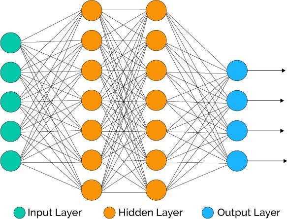
figure 2
Each of these links between neurons has two numbers assigned to it, a weight and a bias. These numbers dictate the relationship between any two neurons – how strongly the activation of one neuron indicates that another in the next layer should be active. To work out the activation of a neuron in a certain layer, the activation of each neuron in the previous layer is multiplied by the weight of their link (which can be positive or negative, indicating whether the linked neurons vary proportionally or inversely), then added to the bias (which can also be positive or negative, and indicates how high the weighted activation needs to be before it becomes meaningful). Once this has been done for each neuron, these numbers are added together, and then passed through a normalisation function such as the sigmoid function (which essentially compresses all its inputs to be between 0 and 1, so that this can become the activation for the new neuron).
Sigmoid Function6:
σ = 1/(1 + e^-x)
Activation Formula7:
α1 = ∑σ(wα0 + b)
Where w the weight, b is the bias, and α1 and α0 represent the activations of neurons in consecutive layers. These weights and biases are assigned randomly for the first run, and as such, the results obtained are random. We can, in this case, imagine the output layer to have ten neurons in it, one for each digit, 0-9. These all contain a number between 0 and 1, representing the probability that any given input is that number – therefore the output neuron with the highest activation is the ANN’s prediction for what number the input represents.
After a first feed forward through the layers, the output we get is random, so to improve the performance of the model we must change the weights and biases in such a way so that the input of a hand-written digit results in the output of the number it represents. To do this we first calculate the “cost function”8 of the algorithm, which is a metric of just how wrong the ANN got its first prediction. We compare the actual result that was obtained through the DL model, which will be ten neurons each containing a random number between 0 and 1, to the results we want to see, which is the correct neuron (the correct neuron being the one that represents the digit that the ML model is looking at) having an activation of 1 and the rest having activations of 0. We then take the MSE of our prediction, by squaring the differences between actual and correct activations so that negative and positive differences don’t cancel out, and averaging thousands of these error values. This forms the cost function of our model. Using calculus, we can work out how exactly to change the input of this function; the weights and biases, in a way that would minimise the output of our function; the cost or error of our model. This changing of the weights and biases to improve the model is known as backpropagation and can be compared to the way in which the brain strengthens the synapses of neurons that fire together – relating to Hebbian Theory. Just like biological neurons learn to associate four legs and four corners with a table, the ANN has learnt to associate the illumination of certain pixels and darkness in others with, for example, the number “3”.
This process of feeding forward followed by backpropagation is a simplified version of the Brain’s central algorithm. Though in recent years more complex formats of neural networks (such as convolutional and recursive NNs) have brought us closer to finding the algorithm of the brain – the concept of a network which learns to recognise patterns by associating observations with higher concepts is identical to the function of the human brain – that is to say, with the right amount of research and innovation, our deep learning algorithms will be able to accurately mimic the brain, leading to machines that are truly intelligent, in the same way that humans are.
Endnotes
figure 1 – https://corochann.com/wp-content/uploads/2017/02/mnist_plot.png
figure 2 – https://cdn-images-1.medium.com/max/800/1*DW0Ccmj1hZ0OvSXi7Kz5MQ.jpeg
2 Hawkins, J. & Blakeslee, S. (2004) On Intelligence. New York, Times Books, Pages 48, 164
3 Kurzweil, R. (2012) How to Create A Mind. USA, Viking Penguin, Page 34
4 Hawkins, J. & Blakeslee, S. (2004) On Intelligence. New York, Times Books
5 Hawkins, J. & Blakeslee, S. (2004) On Intelligence. New York, Times Books, Page 48
6 http://mathworld.wolfram.com/SigmoidFunction.html
7 https://www.youtube.com/watch?v=aircAruvnKk&list=PLZHQObOWTQDNU6R1_67000Dx_ZCJB-3pi&index=2&t=24s
8 https://www.youtube.com/watch?v=IHZwWFHWa-w&t=439s&index=3&list=PLZHQObOWTQDNU6R1_67000Dx_ZCJB-3pi
Bibliography
- How Alan Turing Invented the Computer Age, Ian Watson, 26 April 2012: https://blogs.scientificamerican.com/guest-blog/how-alan-turing-invented-the-computer-age/
- Deep learning in neural networks: An overview, Jürgen Schmidhuber, January 2015: https://www.sciencedirect.com/science/article/pii/S0893608014002135#a000005
- Neural Networks Demystified, Welch Labs, 4 November 2014: https://www.youtube.com/watch?v=bxe2T-V8XRs&list=PLiaHhY2iBX9hdHaRr6b7XevZtgZRa1PoU
- Hawkins, J. & Blakeslee, S. (2004) On Intelligence. New York, Times Books
- Hebbian Theory https://www.sciencedirect.com/topics/neuroscience/hebbian-theory
- Summary of ‘Computing Machinery And Intelligence’ (1950) by Alan Turing, 22 March 2015: http://www.jackhoy.com/artificial-intelligence/2015/03/22/summary-of-computing-machinery-and-intelligence-alan-turing.html
- This Canadian Genius Created Modern AI, Bloomberg, 25 January 2018: https://www.youtube.com/watch?v=l9RWTMNnvi4
- A ‘Brief’ History of Neural Nets and Deep Learning, 24 December 2015: http://www.andreykurenkov.com/writing/ai/a-brief-history-of-neural-nets-and-deep-learning/
- MNIST dataset introduction: https://corochann.com/mnist-dataset-introduction-1138.html
- Machine learning fundamentals (II): Neural networks: https://towardsdatascience.com/machine-learning-fundamentals-ii-neural-networks-f1e7b2cb3eef
- How transferable are features in deep neural networks? http://papers.nips.cc/paper/5347-how-transferable-are-features-in-deep-n%E2%80%A6
- Kurzweil, R. (2012) How to Create A Mind. USA, Viking Penguin
- When to Use MLP, CNN, and RNN Neural Networks, Jason Brownlee, 23 July 2018: https://machinelearningmastery.com/when-to-use-mlp-cnn-and-rnn-neural-networks/
- But what *is* a Neural Network? | Deep learning, chapter 1, 3Blue1Brown, 5 October 2017: https://www.youtube.com/watch?v=aircAruvnKk&list=PLZHQObOWTQDNU6R1_67000Dx_ZCJB-3pi&index=2&t=24s
- Gradient descent, how neural networks learn | Deep learning, chapter 2, 3Blue1Brown, 16 October 2017:
https://www.youtube.com/watch?v=IHZwWFHWa-w&t=439s&index=3&list=PLZHQObOWTQDNU6R1_67000Dx_ZCJB-3pi
- What is backpropagation really doing? | Deep learning, chapter 3, 3Blue1Brown, 3 November 2017:
https://www.youtube.com/watch?v=Ilg3gGewQ5U&t=355s&index=4&list=PLZHQObOWTQDNU6R1_67000Dx_ZCJB-3pi